2.1 Scheduled Commercial Banks

(a) Banking stability indicator (BSI) and map

The banking stability map and indicator present an overall assessment of changes in underlying conditions and risk factors that have a bearing on the stability of the banking sector during a period. The six composite indices represent risk in six dimensions - soundness, asset quality, profitability, liquidity, efficiency and sensitivity to market risk. Each composite index is a relative measure of risk during the sample period used for its construction, where a higher value would mean higher risk in that dimension.

The financial ratios used for constructing each composite index are given in Table 1. Each financial ratio is first normalised for the sample period using the following formula:

where X_t is the value of the ratio at time t. If a variable is negatively related to risk, then normalisation is done using 1-Y_t. Composite index of each dimension is then calculated as a simple average of the normalised ratios in that dimension. Finally, the banking stability indicator is constructed as a simple average of these six composite indices. Thus, each composite index and the overall banking stability indicator takes values between zero and one.

(b) Macro stress test

Macro stress test evaluates the resilience of banks against adverse macroeconomic shocks. It attempts to assess the impact on capital ratios of banks¹ over a one-and-half to two-year horizon, under a baseline and two adverse scenarios. The test encompasses credit risk, market risk and interest rate risk in the banking book. The salient features are as below:

I. Macro-scenario design: The test envisages three scenarios - a baseline and two hypothetical adverse macro scenarios. While the baseline scenario is derived from the forecasted path of select macroeconomic variables, the two adverse scenarios are derived based on hypothetical stringent stress scenario narratives and by performing simulations using the following Vector Autoregression with Exogenous Variables (VARX) model,

with GDP growth, CPI inflation, repo rate and lending spread as the endogenous variables and US GDP growth and US-VIX as exogeneous variables.

II. Projection of key financial variables: Slippage ratio, interest income and interest expense are projected at bank-level using panel regression models for each bank group. GNPA ratio and provision are projected using structural models. Non-interest income [comprising of (a) fee income and (b) other operating income excluding fee income] and non-interest expense are projected based on assumed growth rate of these variables under each scenario.

(i) Projection of slippage ratio: The quarterly slippage ratios at bank level are projected using the following panel regression model;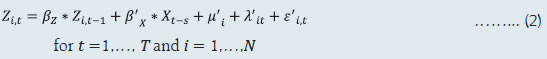

Z_i,t is the quarterly slippage ratio of bank i during quarter t, X_t is a vector of macroeconomic variables including lending spread and GDP growth, μ'_i represents bank-specific fixed effects, λ'_it represents adjustments for specific quarters and ε'_i,t is an i.i.d. error term. Subsequently, quarterly slippage ratios, Ẑ_i,t s are computed based on first differences of the regression equation (2) as,

(ii) Projection of gross loans and advances: Bank level gross loans and advances are projected by applying growth rate equivalent to nominal GDP growth as,

where L_i,t represents the gross loans and advances of bank i at the end of quarter t, and g_t represents the nominal GDP growth rate during quarter (t-1, t).

(iii) Projection of non-performing loans (NPL) or GNPAs: Bank-level GNPAs are projected using the equation,

where NPL_i,t represents the stock of GNPA of bank i at the end of quarter t, WRO_i,t, CURER_i,t and RECRi,t are write-off, upgradation and recovery rates of bank i during the quarter t respectively, PD_i,t is the probability of default (slippage ratio) projected in (3) and PL_i,t-1 is the stock of performing loans at the end of quarter t-1.

(iv) Projection of performing loans (PL): The stock of performing loans for bank i at the end of quarter t, PL_i,t is projected as,

(v) Projection of provisions: Provisions of bank i for quarter t are projected as follows,

where provisioning coverage ratio (PCR) is assumed at 75 per cent. The loss given default (LGD) during quarter t is derived based on the model of Frye and Jacobs (2012), as below

and the parameter k is derived as,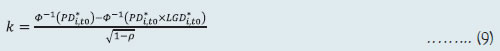

PD* and LGD* are long-term average PDs and LGDs and Φ represents the cumulative normal distribution function.

(vi) Projection of interest income and expenses: Interest income (as share of interest-earning assets) and interest expenses (as share of interest-bearing liabilities) are modelled as functions of macroeconomic variables (GDP growth and call rate) and bank fixed effects with structure similar to equation (2). Bank-wise projections of these ratios are applied to derive shocks to yield on assets and cost of funds for each bank.

(vii) Projection of market risk: Market risk is estimated by applying MTM revaluation of bond exposures (AFS and HFT portfolio) of banks using three inputs, (i) bond exposure, (ii) Macaulay duration, and (iii) interest rate shock, using the bond revaluation formula:

where D is the Macaulay duration, r is the risk-free rate, s is credit spread component, t is the time steps until maturity T, V is the market value, Δr_t+1 represents the risk-free rate shift and Δs_t+1 the credit spread shift. Further, equity and foreign exchange risk are also factored into market risk.

(viii) Projection of net profit: Net profit is projected as,

(ix) Projection of capital: Capital is projected as,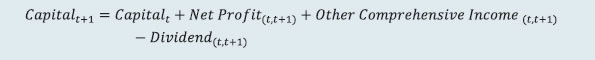

(x) Projection of risk weighted assets (RWA): RWA for Credit risk is projected as,

where g_t represents the nominal GDP growth rate during the period (t, t+1).

RWA for market risk and RWA for operational risk are also projected to grow at nominal GDP growth rate.

III. Major assumptions: Provisions for income tax are assumed at 30 per cent, 30 per cent and 35 per cent of profit before tax for public sector banks (PSBs), private sector banks (PVBs) and foreign banks (FBs), respectively. Dividend payout ratio is assumed at 35 per cent of net profit. Balance sheet is projected to grow at the rate of nominal GDP growth.

(c) Single factor sensitivity analysis – Stress testing

As part of quarterly surveillance, stress tests are conducted covering credit risk, interest rate risk, liquidity risk, equity price risk. and the resilience of scheduled commercial banks (SCBs) in response to these shocks is studied. The analysis is done on individual SCBs as well as on the system level.

I. Credit risk (includes concentration risk)

To ascertain the resilience of banks, the credit portfolio was given a shock by increasing GNPA ratio for the entire portfolio. For testing the credit concentration risk, default of the top individual borrower(s) and the largest group borrower(s), in terms of credit outstanding, was assumed. The analysis was carried out both at the aggregate level as well as at the individual bank level. In case of credit risk, the assumed increase in GNPAs was distributed across sub-standard, doubtful and loss categories in the same proportion as prevailing in the existing stock of GNPAs at system level. However, for credit concentration risk (exposure based), the additional GNPAs under the assumed shocks were considered to fall into sub-standard category only and for credit concentration risk (stressed advances based), stressed advances were considered to fall into loss category. The provisioning requirements were taken as 25 per cent, 75 per cent and 100 per cent for sub-standard, doubtful and loss advances, respectively. These norms were applied on additional GNPAs calculated under a stress scenario. As a result of the assumed increase in GNPAs, loss of income on the additional GNPAs for one quarter was also included in total losses, in addition to the incremental provisioning requirements. The estimated provisioning requirements so derived were deducted from banks’ capital and the capital adequacy ratios under stress scenarios were computed.

II. Sectoral credit risk

To ascertain the sectoral credit risk of individual banks, the credit portfolios of a particular sector was given a shock by increasing GNPA ratio for the sector, based on standard deviation (SD) of GNPA ratios of the sector. The additional GNPAs under the assumed shocks were considered to fall into sub-standard category only. Calculation of the impact on capital is similar to that of stress test for credit risk described above.

III. Interest rate risk

Under assumed shocks of shift in the INR yield curve, there could be losses on account of the fall in value of the portfolio or decline in income.

For interest rate risk in the investment portfolio: AFS, FVTPL (including HFT book) and HTM categories, a duration analysis approach was considered for computing the valuation impact (portfolio losses). The portfolio losses on these investments were calculated for each time bucket of AFS, FVTPL (including HFT book) and HTM categories based on the applied shocks. These estimated losses were reduced from banks’ capital and market risk weighted losses from RWA to arrive at capital ratios under stress scenarios.

Interest rate risk of banks refers to the risk to a bank’s capital and earnings arising from adverse movements in interest rates that affect bank’s books. The impact on earnings is measured using the traditional gap analysis (TGA) and the capital impact is measured by duration gap analysis (DGA). The focus of TGA is to measure the level of a bank’s exposure to interest rate risk in terms of the sensitivity of its net interest income (NII) to interest rate movements over one-year horizon. It involves bucketing of all rate-sensitive assets (RSA), rate-sensitive liabilities (RSL), and off-balance sheet items as per residual maturity / re-pricing date, in various time bands and computing earnings-at-risk (EAR) i.e., loss of income under different interest rate scenarios over a time horizon of one year. Advances, investments, swaps / forex swaps and reverse repos are the major contributors to RSA whereas deposits, swaps / forex swaps and repos are the main elements under RSL. The DGA involves bucketing of all RSA and RSL as per residual maturity / re-pricing dates in various time bands and computing the modified duration gap (MDG) to estimate the impact on the market value of equity. MDG is calculated with the following formula: MDG = [MDA - MDL * (RSL / RSA)], where MDA and MDL are the weighted averages of the modified duration (MD) of items of RSA and RSL, respectively. Thereafter, change in market value of equity (MVE) is computed as ΔE/ E = -[MDG]*RSA* Δi/ E, where Δi is the change in interest rate and E is equity (i.e. net worth).

IV. Equity price risk

Under the equity price risk, the impact of the shock of a fall in the equity price index, by certain percentage points, on bank capital was examined. The loss due to the fall in the value of the portfolio on account of change in equity prices is deducted from the bank’s capital to arrive at the capital under stress scenarios.

V. Liquidity risk

Liquidity stress test assesses the ability of a bank to withstand unexpected liquidity drain without taking recourse to any outside liquidity support. The stress test is based on the Liquidity Coverage Ratio (LCR) framework. The baseline scenario for the stress test depicts the extant LCR computation guidelines and accordingly applies weights used for LCR computation, to each component of cash outflows, inflows and liquid assets. The adverse stress scenarios are designed by applying higher run-off rates relative to the baseline scenario to certain cash outflows (Table 2). LCR for each bank is computed under each of these scenarios.

(d) Bottom-up stress testing: Credit, market and liquidity risks

Bottom-up sensitivity analyses for credit, market and liquidity risks were performed by 37 select scheduled commercial banks. A set of common stress scenarios and shocks were provided to the select banks. The tests were conducted by the banks using relevant data at end-March 2025 and their own methodologies for calculating losses in each case.

(e) Bottom-up stress testing: Derivatives portfolios of select banks

Stress tests on derivatives portfolio (in terms of notional value) were carried out by a sample of 36 banks, constituting the major active authorised dealers and interest rate swap counterparties. Each bank in the sample was asked to assess the impact of stress conditions on their respective derivatives portfolio.

In case of domestic banks, the derivatives portfolio of both domestic and overseas operations was included. In case of foreign banks, only the domestic (Indian) position was considered for the exercise. Derivatives trades where hedge effectiveness was established were exempted from the stress tests, while all other trades were included.

The stress scenarios incorporated four shocks consisting of the spot USD-INR rate and domestic interest rates as parameters (Table 3).

2.2 Primary (Urban) Co-operative Banks

Single factor sensitivity analysis – Stress testing

Stress testing of UCBs was conducted with reference to the reported position as of March 2025. The banks were subjected to baseline, medium and severe stress scenarios in the areas of credit risk, market risk and liquidity risk as follows:

I. Credit default risk

• Under credit default risk, the model aims to assess the impact of stressed credit portfolio of a bank on its CRAR.

• The arithmetic mean of annual growth rate of GNPAs was calculated separately for each NPA class (sub-standard, doubtful 1 (D1), doubtful 2 (D2), doubtful 3 (D3) and loss assets) based on reported data between 2009 and 2024 for the UCB sector as a whole. This arithmetic mean of annual growth rate formed the baseline stress scenario, which was further stressed by applying shocks of 1.5 standard deviation (SD) and 2.5 SD to generate medium and severe stress scenarios for each category separately. These were further adjusted based on NPA divergence level.

• Based on the above methodology, the annual NPA growth rate matrix arrived at under the three scenarios are as below.

II. Credit concentration risk

• The impact of CRAR, under assumed scenarios of top 1, 2, 3 single borrower exposures moving to ‘loss advances’ category, requiring 100 per cent provisioning, was assessed. These exposures may not necessarily be ‘standard advances’ but are identified based on their potential to require higher provisioning, thereby reflecting more impactful stress scenario.

III. Interest rate risk in trading book

• Duration analysis approach was adopted for analysing the impact of upward movement of interest rates on the AFS and HFT portfolio of UCBs.

• Upward movement of interest rates by 50 bps, 100 bps and 150 bps were assumed under the three stress scenarios and consequent provisioning impact on CRAR was assessed.

IV. Interest rate risk in banking book

• The banking book of UCBs was subjected to interest rate shocks of 50 bps, 100 bps and 150 bps under three stress scenarios and its impact on net interest income was assessed.

V. Liquidity risk

• The stress test was conducted based on cumulative cash flows in the 1-28 days’ time bucket. The cash inflows and outflows were stressed under baseline, medium, and severe scenarios.

• While the inflows are stressed uniformly at 5 per cent under all the stress scenarios, outflows are stressed based on worst negative deposit growth recorded across quarters for the periods ranging across past ten years (2014 - 2024). Since UCBs are primarily dependent on deposits as major source of funds, negative growth in deposits is considered as representative of stressed outflows. Further, three months period is considered as representative of 1-28 days’ bucket as this is the closest short-term period for which deposits data is available for all the banks (given that all the banks submit quarterly returns). The average of worst negative deposit growth rate for ten years is considered as baseline scenario, which is further stressed by 1.5 SD and 2.5 SD to generate medium and severe stress scenarios for outflows.

• The banks with negative cumulative mismatch (cash inflow less cash outflow) exceeding 20 per cent of the outflows were considered to be under stress on the basis of the circular RBI/2008-09/174 UBD. PCB. Cir. No12/12.05.001/2008-09 dated September 17, 2008, which stipulates that the mismatches (negative gap between cash inflows and outflows) during 1-14 days and 15-28 days’ time bands in the normal course should not exceed 20 per cent of the cash outflows in each time band.

2.3 Non-Banking Financial Companies (NBFCs)

(a) Non-banking stability indicator (NBSI) and map

The non-banking financial company (NBFC) stability indicator (NBSI) presents an overall assessment of changes in underlying conditions and risk factors that have a bearing on the stability of the NBFC sector during a period. In line with the scale-based regulatory structure, NBFCs falling in the upper and middle layers (excluding the Core Investment Companies (CICs), Primary Dealers (PDs) and Housing Finance Companies (HFCs)) have been considered for construction of the indicator and a related stability map.

The NBSI constitutes five composite indices representing risks in five dimensions – soundness, asset-quality, profitability, liquidity and efficiency. Each composite index is a relative measure of risk and is constructed using multiple financial ratios in respective risk dimension (Table 4). A higher value of a composite index would mean higher risk in that dimension.

Each financial ratio is first normalized for the sample period using the following formula:

where X_t is the value of the financial ratio at time t. If a variable is negatively related to risk, then it is normalized using 1-Y_t. Composite index of each dimension is then calculated as a simple average of the normalized ratios in that dimension. Finally, the NBSI is constructed as a simple average of these five composite indices. Each composite index and the overall NBSI take values between zero and one.

(b) Single factor sensitivity analysis - Stress testing

Credit and liquidity risk stress tests for NBFCs have been performed under baseline, medium and high risk scenarios.

I. Credit risk

Major items of the balance sheet of NBFCs over one year horizon were projected by applying moving average and smoothing techniques. Assets, advances to total assets ratio, earnings before profit and tax (EBPT) to total assets ratio, risk-weight density and slippage ratio were projected over the next one year; and thereafter, based on these projections – new slippages, provisions, EBPT, risk-weighted assets and capital were calculated for the baseline scenario. For the medium and high-risk scenarios, GNPA ratios under baseline scenario were increased by 1 SD and 2 SD and accordingly revised capital and CRAR were calculated.

II. Liquidity risk

Cash flows under stress scenario and mismatch in liquidity position were calculated by assigning assumed percentage of stress to the overall cash inflows and outflows in different time buckets over the next one year. Projected outflows and inflows over the next one year were considered for calculating the liquidity mismatch under the baseline scenario. Outflows and inflows of the sample NBFCs were applied a shock of 5 per cent and 10 per cent for time buckets over the next one year for the medium and high-risk scenarios, respectively. Cumulative liquidity mismatch due to such shocks were calculated as per cent of cumulative outflows and, NBFCs with negative cumulative mismatch were identified.

2.4 Stress Testing Methodology of Mutual Funds

The SEBI has mandated all open-ended debt schemes (except overnight schemes) to conduct stress testing. Accordingly, Association of Mutual Funds in India (AMFI) prescribed the “Best Practice Guidelines on Stress Testing by Debt Schemes of Mutual Funds”. The stress testing is carried out internally by all Asset Management Companies (AMCs) on a monthly basis and also when the market conditions require so. A uniform methodology is being followed across the industry for stress testing with a common outcome, i.e., impact on NAV as a result of the stress testing.

Stress testing parameters

The stress testing is conducted on the three risk parameters, viz., interest rate risk, credit risk and liquidity risk.

(a) Interest rate risk parameter

For interest rate risk parameter, AMCs subject the schemes at portfolio level to the following scenarios of interest rate movements and assess the impact on NAV.

1. The highest increase in G-Sec yield in the last 120 months (1-year G-Secs or 10-year G-Secs whichever is higher on month-on-month basis comparing maximum yield of a month to minimum yield of previous month).

2. Two-third of the highest increase in G-Sec yield in the last 120 months.

3. One-third of the highest increase in G-Sec yield in the last 120 months

(b) Credit risk parameter

For credit risk parameter, AMCs may subject the securities held by the scheme to the following:

1. Calculate the probability of downgrade of each security. In this regard, to incorporate all possible downgrade scenarios (notches) for each security, probability tables published by rating agencies are being used.

2. Further, each potential notched down rating will correspond to a change in valuation yield for the security corresponding to that change in rating. The change in valuation yields for the respective rating changes is derived from the valuation matrix used by the valuation agencies.

3. The sum product of probability of downgrade within investment grade and change in yield on that downgrade of a security, is then multiplied by the duration of that security and the weightage of that security in the portfolio. Separately, the sum product of probability of downgrade below investment grade with haircut applicable on that downgrade of any security, is multiplied with the weightage of that security in the portfolio. These two sum products are added to get the aggregate potential impact at a security level.

4. The summation of all these security level outputs is considered as the portfolio level credit impact.

(c) Liquidity risk parameter

For liquidity risk parameter, the following analysis is being undertaken:

1. Data for past periods of stress (viz. stress scenarios during the years 2008, 2013, 2018, 2020) along with rise in yields for a given credit rating, type of security, etc. in respective matrices for the relevant duration bucket is considered.

2. The change in median yield differential over G-Sec during stress period compared to the preceding normal period (normal period is a period starting 6 months prior to the start of the stress period and ending at the start of the stress period) is considered as rise in spread for the purpose of stress testing.

3. AMCs take yield spike as higher than the AMFI-specified values for stress testing based on market scenarios.

4. These calculations are again reiterated for individual securities based on respective ratings, matrix-based sector as provided in the matrix files and duration bucket and aggregated at the portfolio level to get the portfolio level output.

AMCs additionally consider extreme stress scenarios of time bound liquidation (viz 5 days, 3 days and 1 day) of full portfolios and its impact on NAV by applying suitable haircuts.

2.5 Methodology for Stress Testing Analysis at Clearing Corporations

The SEBI has specified the granular norms related to core settlement guarantee fund (SGF); stress testing and default procedures to create a core fund (called core SGF) within the SGF against which no exposure is given and which is readily and unconditionally available to meet settlement obligations of clearing corporation in case of clearing member(s) failing to honour settlement obligation; align stress testing practices of clearing corporations with Principles for Financial Market Infrastructures (norms for stress testing for credit risk, stress testing for liquidity risk and reverse stress testing including frequency and scenarios); capture the risk due to possible default in institutional trades in stress testing; harmonise default waterfalls across clearing corporations; limit the liability of non-defaulting members in view of the Basel capital adequacy requirements for exposure towards central counterparties (CCPs); ring-fence each segment of clearing corporation from defaults in other segments; and bring in uniformity in the stress testing and the risk management practices of different clearing corporations especially with regard to the default of members.

Stress testing is carried out at clearing corporations (CCs) to determine the minimum required corpus (MRC), which needs to be contributed by clearing members (CMs) to the core SGF. The MRC is determined separately for each segment (viz. cash market, equity derivatives, currency derivatives, commodity derivatives, debt and tri-party repo segment) every month based on stress testing subject to the following:

1. The MRC is fixed for a month.

2. By 15th of every month, CCs review and determine the MRC for next month based on the results of daily stress tests of the preceding month.

3. For every day of the preceding month, uncovered loss numbers for each segment are estimated based on stress test and highest of such numbers is taken as worst-case loss number for the day.

4. Average of all the daily worst case loss numbers determined in (iii) above is calculated.

5. The MRC for next month is at least the higher of the average arrived in at step (iv) above and the segment MRC as per previous review.

For determining the MRC for cash, equity derivatives and currency derivatives segment, CCs calculate the credit exposure arising out of a presumed simultaneous default of top two CMs. The credit exposure for each CM is determined by assessing the close-out loss arising out of closing open positions (under stress testing scenarios) and the net pay-in/ pay-out requirement of the CM against the required margins and other mandatory deposits of the CM. The MRC or average stress test loss of the month is determined as the average of all daily worst case loss scenarios of the month. The actual MRC for any given month is determined as at least the higher of the average stress test loss of the month or the MRC arrived at any time in the past. For the debt segment, the trading volume is minimal, and hence the MRC for the core SGF is calculated as higher of ₹4 crore or aggregate losses of top two CMs, assuming close out of obligations at a loss of four per cent less required margins. The tri-party repo segment and commodity derivatives segment also follow the same stress testing guiding principles as prescribed for equity cash, equity derivatives and currency derivatives segments. For commodity derivatives segment, however, MRC is computed as the maximum of either credit exposure on account of the default of top two CMs or 50 per cent of credit exposure due to simultaneous default of all CMs. Further, the minimum threshold value of MRC for commodity derivatives segment of any stock exchange is ₹10 crore.

CCs carry out daily stress testing for credit risk using at least the standardized stress testing methodology prescribed by SEBI for each segment. Apart from the stress scenarios prescribed for cash market and derivatives market segments, CCs also develop their own scenarios for a variety of ‘extreme but plausible market conditions’ (in terms of both defaulters’ positions and possible price changes in liquidation periods, including the risk that liquidating such positions could have an impact on the market) and carry out stress testing using self-developed scenarios. Such scenarios include relevant peak historic price volatilities, shifts in other market factors such as price determinants and yield curves, multiple defaults over various time horizons and a spectrum of forward-looking stress scenarios in a variety of extreme but plausible market conditions. Also, for products for which specific stress testing methodology has not been prescribed, CCs develop extreme but plausible market scenarios (both hypothetical and historical) and carry out stress tests based on such scenarios and enhance the corpus of SGF, as required by the results of such stress tests.

2.6 Interconnectedness – Network Analysis

Matrix algebra is at the core of the network analysis, which uses the bilateral exposures between entities in the financial sector. Each institution’s lending to and borrowings from all other institutions in the system are plotted in a square matrix and are then mapped in a network graph. The network model uses various statistical measures to gauge the level of interconnectedness in the system. Some of the important measures are given below: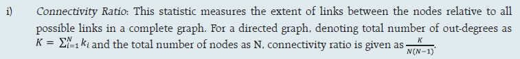

ii) Cluster coefficient: Clustering in networks measures how interconnected each node is. Specifically, there should be an increased probability that two of a node’s neighbours (banks’ counterparties in case of a financial network) are neighbours to each other also. A high clustering coefficient for the network corresponds with high local interconnectedness prevailing in the system. For each bank with k_i neighbours the total number of all possible directed links between them is given by k_i(k_i-1). Let E_i denote the actual number of links between bank i’s k_i neighbours. The clustering coefficient C_i for bank i is given by the identity:

The clustering coefficient (C) of the network as a whole is the average of all C_i’s:

iii) Tiered network structures: Typically, financial networks tend to exhibit a tiered structure. A tiered structure is one where different institutions have different degrees or levels of connectivity with others in the network. In the present analysis, the most connected banks are in the innermost core. Banks are then placed in the mid-core, outer core and the periphery (the respective concentric circles around the centre in the diagram), based on their level of relative connectivity. The range of connectivity of the banks is defined as a ratio of each bank’s in-degree and out-degree divided by that of the most connected bank. Banks that are ranked in the top 10 percentile of this ratio constitute the inner core. This is followed by a mid-core of banks ranked between 90 and 70 percentile and a 3rd tier of banks ranked between the 40 and 70 percentile. Banks with a connectivity ratio of less than 40 per cent are categorised in the periphery.

iv) Colour code of the network chart: The blue balls and the red balls represent net lender and net borrower banks respectively in the network chart. The colour coding of the links in the tiered network diagram represents the borrowing from different tiers in the network (for example, the green links represent borrowings from the banks in the inner core).

(a) Solvency contagion analysis

The contagion analysis is in the nature of a stress test where the gross loss to the banking system owing to a domino effect of one or more banks failing is ascertained. We follow the round by round or sequential algorithm for simulating contagion that is now well known from Furfine (2003). Starting with a trigger bank i that fails at time 0, we denote the set of banks that go into distress at each round or iteration by Dq, q = 1,2, …For this analysis, a bank is considered to be in distress when its Tier I capital ratio goes below 7 per cent. The net receivables have been considered as loss for the receiving bank.

(b) Liquidity contagion analysis

While the solvency contagion analysis assesses potential loss to the system owing to failure of a net borrower, liquidity contagion estimates potential loss to the system due to the failure of a net lender. The analysis is conducted on gross exposures between banks comprising both fund based ones and derivatives. The basic assumption for the analysis is that a bank will initially dip into its liquidity reserves or buffers to tide over a liquidity stress caused by the failure of a large net lender. The items considered under liquidity reserves are: (a) excess CRR balance; (b) excess SLR balance; and (c) 18 per cent of NDTL. If a bank is able to meet the stress with liquidity buffers alone, then there is no further contagion.

However, if the liquidity buffers alone are not sufficient, then a bank will call in all loans that are ‘callable’, resulting in a contagion. For the analysis only short-term assets like money lent in the call market and other very short-term loans are taken as callable. Following this, a bank may survive or may be liquidated. In this case there might be instances where a bank may survive by calling in loans, but in turn might propagate a further contagion causing other banks to come under duress. The second assumption used is that when a bank is liquidated, the funds lent by the bank are called in on a gross basis (referred to as primary liquidation), whereas when a bank calls in a short-term loan without being liquidated, the loan is called in on a net basis (on the assumption that the counterparty is likely to first reduce its short-term lending against the same counterparty. This is referred to as secondary liquidation).

(c) Joint solvency-liquidity contagion analysis

A bank typically has both positive net lending positions against some banks while against some other banks it might have a negative net lending position. In the event of failure of such a bank, both solvency and liquidity contagion will happen concurrently. This mechanism is explained by the following flowchart:

The trigger bank is assumed to have failed for some endogenous reason, i.e., it becomes insolvent and thus impacts all its creditor banks. At the same time it starts to liquidate its assets to meet as much of its obligations as possible. This process of liquidation generates a liquidity contagion as the trigger bank starts to call back its loans.

Since equity and long-term loans may not crystallise in the form of liquidity outflows for the counterparties of failed entities, they are not considered as callable in case of primary liquidation. Also, as the RBI guideline dated March 30, 2021 permits the bilateral netting of the MTM values in case of derivatives at counterparty level, exposures pertaining to derivative markets are considered to be callable on net basis in case of primary liquidation.

The lender / creditor banks that are well capitalised will survive the shock and will generate no further contagion. On the other hand, those lender banks whose capital falls below the threshold will trigger a fresh contagion. Similarly, the borrowers whose liquidity buffers are sufficient will be able to tide over the stress without causing further contagion. But some banks may be able to address the liquidity stress only by calling in short term assets. This process of calling in short term assets will again propagate a contagion.

The contagion from both the solvency and liquidity side will stop / stabilise when the loss / shocks are fully absorbed by the system with no further failures.

(d) Identification of impactful and vulnerable banks

Data on bilateral exposures among entities of the financial system are leveraged to compute impact and vulnerability metrics to identify entities that are impactful (causing sizeable capital loss to others in the system upon their default) as well as vulnerable (their own capital loss susceptibility conditional on other entities’ failures), using the following metrics and methodology (IMF, 2017):

(i) Index of contagion (impact) of a bank represents the average loss experienced by other banks (expressed as a percentage of their Tier 1 capital) due to failure of that bank. It is calculated, for bank i, as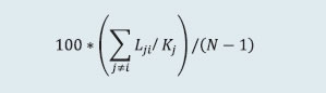

where K_j is bank j’s capital, L_ji is the loss to bank j due to the default of bank i and N is the total number of banks;

(ii) Index of vulnerability of a bank represents the average loss experienced by the bank (expressed as a percentage of its Tier 1 capital) across individually triggered failures of all other banks. It is calculated, for bank i, as

where K_i is bank i’s capital, L_ij is the loss to bank i due to the default of bank j and N is the total number of banks;

(iii) To analyse the effects of a credit shock, the exercise simulates default of each bank with 100 per cent loss-given-default, where the counterparties’ capitals absorb the losses. A bank is said to fail if its Tier 1 capital ratio falls below 7 per cent. In the subsequent rounds, if there are further failures, the losses are aggregated.

The results of indexes calculated can be analysed to identify entities that are common between the set of top highly impactful banks and the set of top highly vulnerable banks.

2.7 Financial System Stress Indicator (FSSI)

FSSI is compiled using risk factors spread across five financial market segments (equity, forex, money, government debt and corporate debt), three financial intermediary segments (banks, NBFCs and AMC-MFs) and the real sector (Table 5). FSSI lies between zero and unity, with higher value indicating more stress. For its construction, the risk factors pertaining to each component segment are first normalised using min-max method and thereafter aggregated based on simple average into a sub-indicator ‘y_i‘ representing the i^th market / sector. Finally, the composite FSSI is obtained as,

where the weight ‘w_i’ of each sub-indicator ‘y_i’ is determined from its sample standard deviation ‘s_i’, as,

¹ The macro stress test is carried out on select 46 scheduled commercial banks (SCBs).